Handwritten Digit Recognition with AI

- Name
- Francisco Sandi
- Published on

During my master’s program, I recently learned about various Deep Learning techniques, with convolutional neural networks (CNNs) standing out due to their effectiveness in image recognition tasks. As a way to solidify my understanding, I decided to play around with the MNIST dataset—a classic in the AI community, often dubbed the "Hello World" of deep learning. In this article, I’ll walk you through the process, the hurdles I faced, and the lessons I learned along the way.
Getting Started
MNIST
The MNIST dataset is a large collection of handwritten digits, commonly used for training various image processing systems. It contains 60,000 training images and 10,000 testing images, each a 28x28 grayscale pixel representation of digits from 0 to 9. Due to its simplicity and well-labeled data, MNIST has become the go-to dataset for anyone beginning their journey in deep learning.
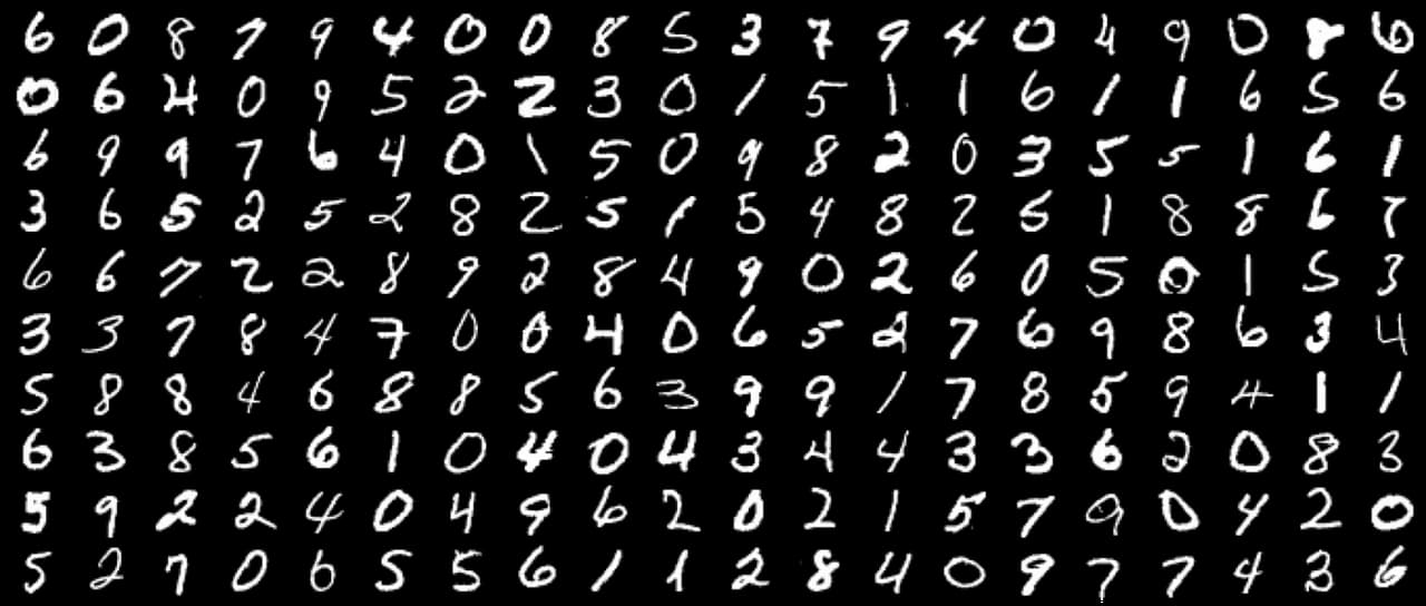
MNIST dataset
Neural Networks (NN)
Neural networks are computational models inspired by the human brain's neural structure. They consist of layers of interconnected nodes, or "neurons," where each connection has an associated weight. The network is trained by adjusting the weights of the connections based on the error in its predictions. This is done through a process called backpropagation, combined with an optimization algorithm like gradient descent. As the network iterates over the data, it gradually learns to make more accurate predictions by minimizing the error.
Convolutional Neural Networks (CNN)
While traditional neural networks are powerful, they have limitations when it comes to handling image data, especially for tasks like digit recognition. CNNs are a specialized type of neural network designed to process data with a grid-like topology, such as images. The key difference between CNNs and traditional NNs lies in the use of convolutional layers, allowing the learning of spatial hierarchies of features, making them exceptionally well-suited for image recognition tasks.
The Experiment
I used PyTorch, a popular Deep Learning framework, to implement and train the Convolutional Neural Network (CNN) on the MNIST dataset. Here’s how I structured the experiment:
Loading Dataset
To prepare the dataset for training and testing, I used PyTorch's DataLoader to efficiently load and organize the MNIST data into batches. Both datasets are loaded in batches of 100 images, with shuffling enabled for the training data to ensure a diverse mix of samples in each batch.
In addition to batching, I applied a series of transformations to the training images to better simulate real-world variations in handwritten digits. Using PyTorch's transforms module, I introduced random rotations, translations, scaling, and shearing to the images. These augmentations help mimic the inconsistency found in actual handwriting, where digits can appear skewed, rotated, or slightly misaligned. This variability forces the model to learn more robust features, improving its ability to generalize to new, unseen data. Furthermore, each image is normalized to have a mean of 0.1307 and a standard deviation of 0.3081, standardizing pixel values to ensure stable and consistent training.
import torch
from torchvision import datasets, transforms

# Training dataset (60000 datapoints)
train_loader = torch.utils.data.DataLoader(
        datasets.MNIST('data', train=True, download=True,
                       transform=transforms.Compose([
                           transforms.RandomAffine(
                               degrees=30, translate=(0.5, 0.5), scale=(0.25, 1),
                               shear=(-30, 30, -30, 30)),
                           transforms.ToTensor(),
                           transforms.Normalize((0.1307,), (0.3081,))
                       ])),
        batch_size=100, shuffle=True)

# Testing dataset (10000 datapoints)
test_loader = torch.utils.data.DataLoader(
        datasets.MNIST('data', train=False, transform=transforms.Compose([
                           transforms.ToTensor(),
                           transforms.Normalize((0.1307,), (0.3081,))
                       ])),
        batch_size=100, shuffle=True)
By applying these transformations, the model becomes more capable of handling real-world handwritten digits, which are rarely as uniform or perfectly centered as the MNIST dataset. Below, you can see an image of a raw dataset sample alongside the corresponding transformed version, showing how these adjustments improve the dataset's diversity and help the model generalize better to real handwriting.
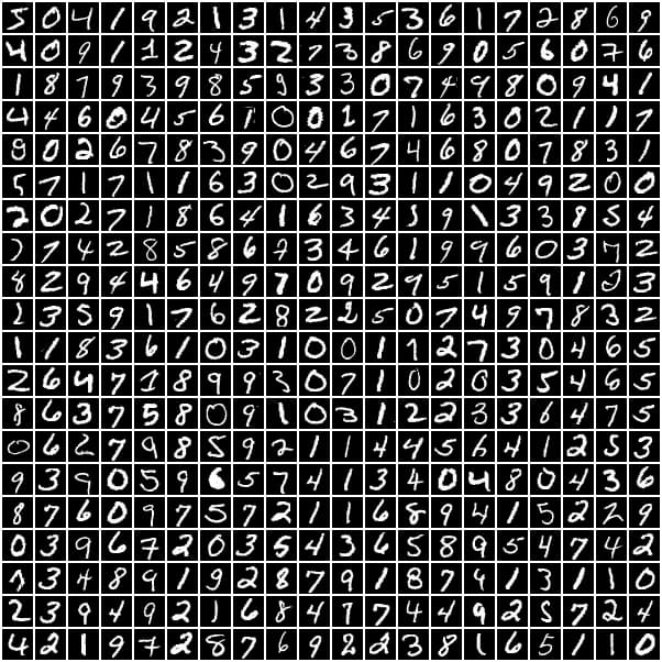
MNIST Dataset Sample
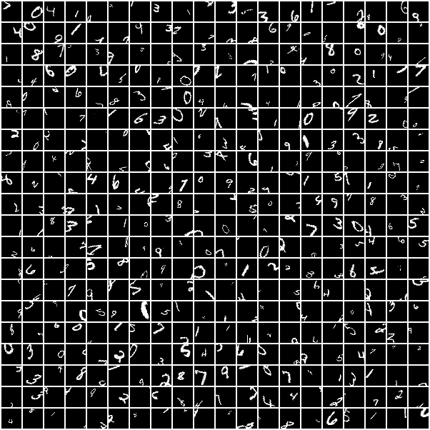
Transformed MNIST Dataset Sample
Defining the Model
The CNN architecture I used was relatively simple but effective for digit recognition. The model consisted of the following layers:
1st convolution: The first layer
conv1, with 16 output channels and a kernel size of 5x5. This design allows the model to capture essential features such as edges and textures from the input grayscale images. Following the convolution, a ReLU activation function is applied, introducing non-linearity that enhances the model's ability to learn complex patterns. Max pooling with a kernel size of 2 further reduces the spatial dimensions, making the model computationally efficient while retaining important feature information.2nd convolution: The second layer
conv2, deepens the model by increasing the number of output channels to 32. This expansion allows for the extraction of more intricate features, enabling the model to recognize more complex patterns in the data. Similar to the first layer, it utilizes a ReLU activation function and max pooling to maintain efficiency and promote effective learning.Fully connected layer: This final layer
outtakes the flattened output from the last convolutional layer and produces predictions for the ten digit classes (digits 0-9).
This structure allowed the model to learn increasingly abstract features of the images as they passed through the layers, from simple edges to more complex shapes.
import torch.nn as nn

class CNN(nn.Module):
    def __init__(self):
        super(CNN, self).__init__()

        # 1st convolutional block
        self.conv1 = nn.Sequential(
            nn.Conv2d(1, 16, 5, 1, 2),  # 1 input channel (grayscale), 16 output channels, 5x5 kernel, stride 1, padding 2
            nn.ReLU(),                  # Activation function (ReLU) introduces non-linearity
            nn.MaxPool2d(2)             # Downsample the feature maps by a factor of 2
        )

        # 2nd convolutional block
        self.conv2 = nn.Sequential(
            nn.Conv2d(16, 32, 5, 1, 2),  # 16 input channels (from conv1), 32 output channels, 5x5 kernel, stride 1, padding 2
            nn.ReLU(),                   # Activation function (ReLU)
            nn.MaxPool2d(2),             # Downsample the feature maps by a factor of 2
        )

        # Fully connected layer
        self.out = nn.Linear(32 * 7 * 7, 10)  # Input size is 32 channels * 7x7 spatial dimensions, output size is 10 classes

    def forward(self, x):
        x = self.conv1(x)          # Pass input through the first convolutional block
        x = self.conv2(x)          # Pass input through the second convolutional block
        x = x.view(x.size(0), -1)  # Flatten the output of conv2 to (batch_size, 32 * 7 * 7)
        output = self.out(x)       # Pass the flattened output through the fully connected layer

        return output, x           # Return the final output and the flattened features
Training
With the model defined, I moved on to training using the following parameters:
- Loss Function: The loss function used is
CrossEntropyLoss, which is ideal for multi-class classification problems. It measures the dissimilarity between the predicted probabilities and the true class labels, guiding the model in minimizing prediction errors. - Optimizer: The
Adamoptimizer is utilized, known for its adaptive learning rate capabilities. It is initialized with a learning rate of 0.01, allowing for effective and efficient updates to the model weights during training. Adam combines the advantages of two other extensions of stochastic gradient descent, improving convergence speed. - Learning Rate Scheduler: A
StepLRscheduler is employed to adjust the learning rate at specified intervals. In this case, the learning rate is reduced by a factor of 0.7 after each epoch. This adjustment promotes stability in learning, helping the model to converge more effectively as training progresses.
The function iterates over batches from the train_loader, transferring both the input data and target labels to the specified device. Each batch undergoes a forward pass through the model to produce predictions, followed by the calculation of the loss. Gradients are cleared, and a backward pass computes the necessary gradients before the optimizer updates the model weights. After processing each epoch, the current loss is printed, providing insights into the model's performance and guiding further adjustments if necessary.
def train(model, device, train_loader, epochs, optimizer, loss_func, scheduler):
    model.train()  # Set the model to training mode
    for epoch in range(1, epochs + 1):  # Loop over the specified number of epochs
        for batch_idx, (data, target) in enumerate(train_loader):  # Iterate over the training data
            data, target = data.to(device), target.to(device)  # Move data and targets to the specified device (GPU/CPU)

            batch_x = Variable(data)  # Create a Variable for input data
            batch_y = Variable(target)  # Create a Variable for target labels

            output = model(batch_x)[0]  # Forward pass: compute model output
            loss = loss_func(output, batch_y)  # Compute the loss

            optimizer.zero_grad()  # Clear previous gradients
            loss.backward()  # Backward pass: compute gradients
            optimizer.step()  # Update model weights based on computed gradients

        scheduler.step()  # Adjust learning rate using the scheduler
        print(f"Epoch {epoch} - Loss: {loss.item():.6f}")  # Print the loss for the current epoch

# Train the model
device = torch.device("cuda" if torch.cuda.is_available() else "cpu")
model = CNN().to(device)
loss_func = nn.CrossEntropyLoss()
optimizer = optim.Adam(model.parameters(), lr = 0.01)
scheduler = StepLR(optimizer, step_size=1, gamma=0.7)
epochs = 15

train(model, device, train_loader, epochs, optimizer, loss_func, scheduler)
Evaluation
The test function evaluates the performance of the trained CNN model on the test dataset. First, the model is set to evaluation mode using model.eval(), ensuring that layers like dropout and batch normalization function appropriately during testing. Two counters, correct and total, track the number of correct predictions and the total samples.
Using torch.no_grad() to disable gradient computation, the function iterates over batches in the test_loader, transferring data and targets to the specified device. A forward pass computes the model's output, and torch.max retrieves the predicted class with the highest probability. The total sample count is updated, and correct predictions are accumulated.
Finally, accuracy is calculated as the percentage of correct predictions, and this metric is printed, providing insight into the model's performance on unseen data.
def test(model, device, test_loader):
    model.eval()  # Set the model to evaluation mode
    correct = 0  # Initialize the counter for correct predictions
    total = 0    # Initialize the counter for total samples

    with torch.no_grad():  # Disable gradient computation during testing
        for data, target in test_loader:  # Iterate over the test data
            data, target = data.to(device), target.to(device)  # Move data and targets to the specified device

            output = model(data)[0]  # Forward pass: compute model output
            _, predicted = torch.max(output.data, 1)  # Get the index of the max log-probability
            total += target.size(0)  # Update total number of samples
            correct += (predicted == target).sum().item()  # Count correct predictions

    accuracy = 100 * correct / total  # Calculate accuracy percentage
    print(f'Accuracy: {accuracy:.2f}%')  # Print the accuracy

test(model, device, test_loader)
In the evaluation phase, the model achieved an impressive accuracy of 98.72% without transformations applied to the training dataset. However, when random affine transformations such as rotation, translation, scaling, and shearing were introduced, the accuracy dropped. This decline is expected, as these transformations add variability, making the model's task more complex. While immediate accuracy may be lower, these transformations are essential for real-world applications. They enhance the model's ability to generalize by training it to handle variations in how handwritten digits might appear, leading to improved robustness and adaptability on unseen data.
Use a real image
After successfully training the CNN on the MNIST dataset, I wanted to see how well it could handle handwritten digits from a real photo. This required several steps to preprocess the data to make it compatible with the model.
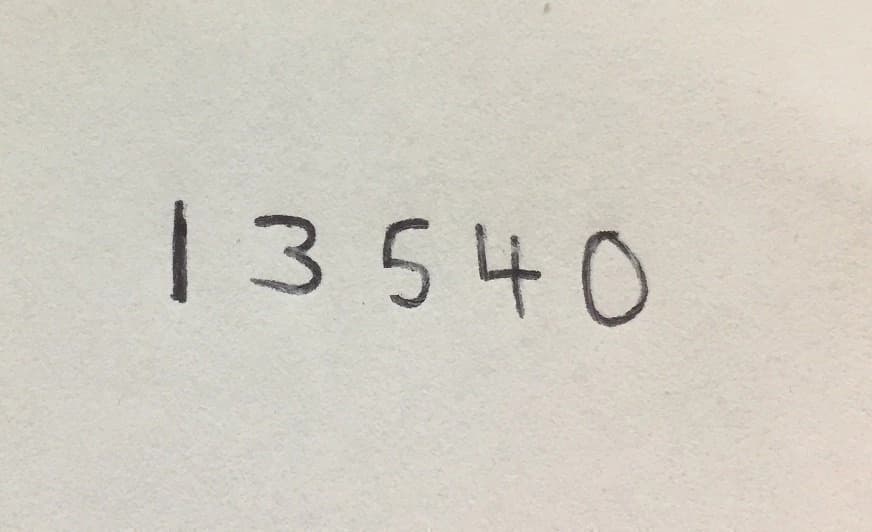
Test image with handwritten digits
Loading & Preprocessing
I began by loading my test image containing handwritten digits using OpenCV. This image was loaded in grayscale to simplify the preprocessing steps. The next step involved extracting individual digits from the image resembling the MNIST dataset. This was very challenging since I don't have much experience with image processing, I'm sure there are betters ways to do this, bit this is the approach I intuitively took:
Binary Format: I converted the image to a binary format using thresholding. This step created a high-contrast binary image where the digits stood out clearly against the background.
Finding Contours: I used contour detection to identify distinct regions in the binary image, each of which potentially contained a digit. These contours were then sorted from left to right to maintain the correct order of digits since my image contains multiple digits.
Remove Noise: To ensure the extracted digits were of a reasonable size, I filtered out contours with small bounding boxes based on the diagonal size of the rectangles.
Padding and Resizing: Each digit was then padded to ensure it had a consistent size and was centered within a square. After padding, the digit images were resized to 28x28 pixels, the same size as the MNIST images, to match the input format expected by the model.
Transformations: Finally, I applied a series of transformations to prepare the digits for model input. This included converting the images to tensors, normalizing them, and maximizing contrast to enhance readability.
Preview Digits: To verify that the preprocessing was done correctly, I previewed the extracted and processed digits. This step was crucial to ensure that the digits were properly preprocessed before feeding them into the model.
import cv2
import math
import torch
import matplotlib.pyplot as plt
import torchvision.transforms as transforms
from PIL import Image

image_path = 'handwritten-numbers.jpg'
image = cv2.imread(image_path, cv2.IMREAD_GRAYSCALE)

# Threshold the image to create a binary image
_, binary_image = cv2.threshold(image, 128, 255, cv2.THRESH_BINARY_INV + cv2.THRESH_OTSU)

# Find contours in the binary image
contours, _ = cv2.findContours(binary_image, cv2.RETR_EXTERNAL, cv2.CHAIN_APPROX_SIMPLE)

# Sort contours from left to right based on the x coordinate of the bounding box
contours = sorted(contours, key=lambda ctr: cv2.boundingRect(ctr)[0])

# Process each contour to get rectangle information
rectangles = [cv2.boundingRect(contour) for contour in contours]

# Filter out rectangles that are too small
maxDiagonal = max([math.sqrt(w**2 + h**2) for (x, y, w, h) in rectangles])
rectangles = [(x, y, w, h) for (x, y, w, h) in rectangles if math.sqrt(w**2 + h**2) > maxDiagonal/2]

# Define the transformation to preprocess the image
transform = transforms.Compose([
    transforms.Grayscale(),  # Convert image to grayscale
    transforms.Resize((28, 28)),  # Resize image to 28x28
    transforms.ToTensor(),  # Convert image to tensor
    transforms.Normalize((0.5,), (0.5,)),  # Normalize the image
    transforms.Lambda(lambda x: torch.where(x > 0.5, torch.ones_like(x), torch.zeros_like(x))) # Maximize contrast
])

digits = []
for (x, y, w, h) in rectangles:
    digit = binary_image[y:y+h, x:x+w]

    # Create a new black square image with padding
    max_dim = max(w, h) + 10
    padded_digit = np.zeros((max_dim, max_dim), dtype=np.uint8)

    # Compute the position to place the original digit in the center
    x_offset = (max_dim - w) // 2
    y_offset = (max_dim - h) // 2

    # Place the original digit image in the center of the new image
    padded_digit[y_offset:y_offset+h, x_offset:x_offset+w] = digit
    digit = padded_digit
    digit_resized = cv2.resize(digit, (28, 28))

    # Filter out noise, and apply transformations
    min_white_pixels = 50
    if cv2.countNonZero(digit_resized) > min_white_pixels:
      digit_resized = Image.fromarray(digit_resized)
      digit_tensor = transform(digit_resized).unsqueeze(0)
      digits.append((digit_tensor, digit_resized))

# Preview digits obtained from the image
plt.figure(figsize=(10, 2))
for idx, (digit_tensor, digit_image) in enumerate(digits):
    plt.subplot(1, len(digits), idx + 1)
    plt.imshow(digit_image, cmap='gray')
    plt.axis('off')
plt.show()

Extracted digits
Making Predictions
With the digits preprocessed, I loaded the trained CNN model and used it to make predictions on the extracted digits. For each digit, the model produced a prediction, which was then displayed alongside the digit image. This provided a clear view of the model’s performance on the image.
# Make predictions on the extracted digits
model.eval()
predictions = []
plt.figure(figsize=(10, 2))
for idx, (digit_tensor, digit_image) in enumerate(digits):
    output, _ = model(digit_tensor)
    _, predicted = torch.max(output, 1)
    predictions.append(predicted.item())

    # Plot the digit
    plt.subplot(1, len(digits), idx + 1)
    plt.imshow(digit_image, cmap='gray')
    plt.title(f'Pred: {predicted.item()}')
    plt.axis('off')
plt.show()

Results of digit recognition
The predictions were visually confirmed by plotting the digits with their predicted labels. This step allowed me to assess the model’s accuracy and see how well it generalized beyond the MNIST dataset, which surprised me, as at least for this example, all digits were correctly predicted.
Adapting the CNN to handle handwritten digits from a picture involved several preprocessing steps to convert the image into a format compatible with the trained model. This process demonstrated some of the practical challenges of working with real-world data and highlighted the importance of robust image preprocessing techniques.
However, when I tested the model with images containing less clear digits or those affected by shadows and varying lighting conditions, the results were less accurate. This indicates that further preprocessing and potentially more advanced techniques may be necessary to improve performance in real-world applications, where variability in digit quality and image conditions can significantly impact recognition accuracy.
Try It Yourself
To give you a hands-on experience with the trained model, I’ve created a web utility in the site where you can draw your own numbers and see how well the model recognizes them. This interactive tool lets you play around with the trained CNN and see its predictions in real-time.
Feel free to experiment with different numbers and see how accurately the model can identify them. You can access the tool 👉 here.

AI Digit Recognition Tool
I hope you enjoy exploring the model's capabilities and find it helpful for understanding how convolutional neural networks can be used for image recognition!
Resources
- But what is a neural network?: This video inspired me to do this experiment
- Deep Learning Basics: Introductory class to Deep Learning by Lex Friedman
- MNIST dataset: The MNIST database of handwritten digits in Kaggle
- Convolutional Neural Networks: Datacamp introduction to CNNs
If you reached this far, thanks for reading, I hope this was valuable for you in some way. I'm sure readers have very different levels of experience with deep learning, please leave your thoughts in the comments so we all can share what we know and keep learning together.
Previous Article
My First TriathlonNext Article
The Coding Interview